
Five characteristics will underpin commercially viable autonomous-driving (AD) vehicle solutions at Levels 4 and 5: flexibility, high usable compute power, low latency, low power and low cost. The first three are mandatory to implement AD functionality. The last two, while not strictly necessary for meeting the target, are essential for achieving wide and rapid adoption. This article spotlights the technological attributes necessary to realize Level 4/5 autonomy. Legislative and other crucial aspects also figure into the requirements but are not covered here.
From the domain to the zone
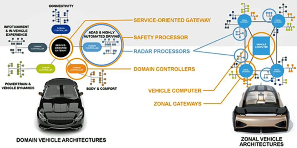
In recent years, architectural designers of vehicle electronics have been redirecting their focus from domain-centric architectures to zonal architectures.
In a domain-centric architecture, a domain control unit handles all functionality related to a specific domain. In automotive applications, examples of functional domains include powertrain and infotainment. They are managed by electronic control units that consist of self-contained functional modules wired to devices and sensors with in-situ computational capabilities.
The domain-centric approach is scalable and efficient as long as devices and sensors are situated close to the module. When the functionality is distributed, however, wiring and interfacing sensors and devices become problematic, increasing cost and lowering reliability.
In a zonal architecture, vehicle functions are grouped by location into several zones. Each zone encompasses the devices installed in that particular section of the vehicle, managed by a local zonal controller or gateway. Because a zonal gateway is close to the devices it controls, the interconnecting cable lengths are short. Each zonal gateway communicates to the central compute unit (CCU) at the heart of the vehicle.
Communication between zonal gateways and the central computer resembles a computer network scheme rather than an automotive harness. This interzonal communication is implemented via a small, high-speed networking cable that reduces the quantity and size of the cables in the vehicle. Zonal architecture offers a scalable, reliable and efficient solution, saving power, weight, material and installation costs (Figure 1).
This architectural shift is consistent with the move to distributed software functionality and the ability to provide enhancements with new software.
An AD vehicle’s central compute unit
The success of a zonal architecture rests on solving the challenges presented to the central compute unit. The CCU enables the five critical attributes, cited earlier, that can make an AD vehicle a reality: flexibility, high compute power, latency, low power and low cost.
Flexibility
AD vehicles are driven by multiple, complex algorithms that are constantly evolving. A flexible—that is, programmable—architecture is a must to accommodate the rapidly changing algorithmic world. With the upcoming software-defined vehicles, an algorithm-agnostic CCU becomes necessary to handle future delivery of new algorithms over the air to the AD vehicle.
In-field programmability is also required to map a new class of algorithms that straddle the barrier between artificial intelligence and digital-signal processing (DSP). For example, in the Mask R-CNN algorithm, some layers require AI processing in 8-bit floating point (fp8), with ResNet50 + FPA functioning as the backbone, whereas other layers require DSP processing (fp16 or fp32).
High compute power
First off, economy of scale dictates a scalable architecture to deliver compute power according to the vehicle class. Typically, the features of an entry-level vehicle are a subset of the full slate of luxury-vehicle features. By using a scalable architecture, software and hardware can be shared across the entire range of vehicles.
“High compute power” is probably one of the most abused terms in the industry right now as companies scramble to show the highest number of operations per second (OPS). For AI processing, compute power is typically measured in trillions of operations per second (TOPS), although most recently, there have been announcements of petaOPS (1 POPS = 1,000 TOPS). This metric provides the maximum theoretical number of operations that a given device can perform when it is occupied 100% of the time. The reality, however, is that the algorithm, and possibly the activation function in the algorithmic processor, will lower the number. The critical and meaningful metric is the number of operations per second that can actually be performed at any given time. This realistic number reflects the architecture of the solution and its implementation efficiency. Most of the time, the usable compute power differs significantly from the maximum theoretical TOPS specified by the supplier.
Low latency
A CCU operates on three stages: perception, (motion) planning and (motion) execution (Figure 2). The perception stage aims at converting the sensory data into a driving scenario consisting of location and environmental conditions to help the CCU formulate a driving path.
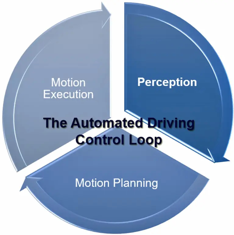
Low latency is critical for successful perception processing. Currently, sensors generate new data every 30 ms, coercing the perception stage to process all data, including error handling, in less than 20 ms. Context awareness also plays a role, as there is a need to get a higher level of environmental understanding for more complex scenarios like executing turns in multilane intersections with cross-traffic that might include cars, trucks, humans, bicycles and streetcars.
The old adage “garbage in, garbage out” holds true here, as the processing of the next stage, motion planning, will be only as good as the results of the perception stage. The same applies to the final stage, motion execution, which sends the necessary signals to the actuators. Because something may still go wrong in the complete control loop, it is necessary to be able to take action on errors within the given loop cycle time.
Low power and low cost
Low power and low cost drive the rapid and broad adoption of the solution. A costly solution would limit the market to the top vehicle class. A power-hungry solution would impact the battery life of an electric vehicle. Further limitations may arise when more complex and more expensive cooling solutions become necessary for high-power–draw implementations.
Low-power and low-cost attributes deal with commercial aspects, whereas flexibility, high processing power and low latency constitute fundamental attributes for implementing AD functionality.
About algorithms and perception
Over time, the algorithms required by L3–L5 self-driving vehicles have dramatically increased in complexity, requiring escalating levels of compute power. While early algorithms like ResNet50, Yolo and Imagenet are still in use today, they have become backbones of new composite and highly complex algorithms, where they have proved useful for benchmarking references.
Transformers, introduced in 2017, have taken over as the foundation for the best and most promising algorithms targeting autonomous vehicles.
As mentioned earlier, performance in the perception stage is critical for mapping the vehicle’s physical surroundings in a 3D geometrical model. One challenge for this accomplishment is to unify into one representation the data collected from the various sensors—camera, radar, LiDAR, ultrasonic, GNSS and odometry, for example. The best candidate for this task is the bird’s-eye–view (BEV) representation. While in 2D, front-view and perspective view (PV) typically are being used; these need to handle issues like occlusion and scaling as part of the process. To get the best performance, the perception stage utilizes a combination of 3D and 2D algorithms, most of which are transformer-based.
Although BEV has been around for a number of years, Tesla spotlighted the technology at its 2021 AI Day. The Tesla approach uses data from eight cameras, feeding the data they collect into an algorithm that generates a fused 3D space with a combination of dynamic (e.g., vehicles, pedestrians) and static (lanes, traffic signs, lights) information. Key information like location, distance, speed, direction and acceleration are also captured (Figure 3).
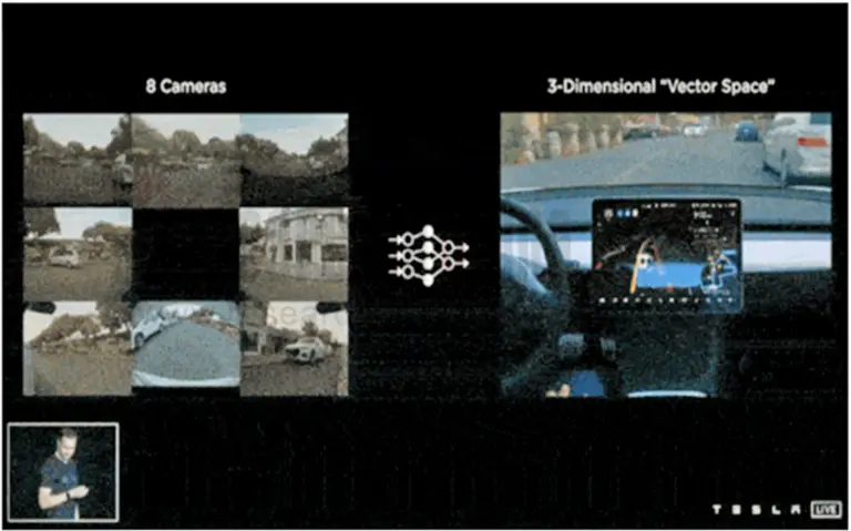
Tesla confirmed that the effectiveness of this solution is limited by the available compute power.
In BEV fusion, added complexity comes into play as the feeds from cameras providing 2D data in PV are combined with those from radar and/or LiDAR units providing 3D data. The process requires the extraction of PV features and their transformation into BEV converted from 2D to 3D. The result is then fused with the features extracted from the 3D data of the point cloud, as an example. The procedure maintains the most original information for a more accurate perception result. Unfortunately, this is achieved at the expense of increased compute power to meet the low-latency requirements. BEV today is one of the key drivers in algorithm development.
Another successful and promising algorithm is the particle filter, a DSP algorithm used in dynamic occupancy grid mapping (abbreviated as DOGMa). The traditional way to start the perception process has been to use a grid map to estimate the cell occupancy and understand the environment around the vehicle. The classical occupancy maps were based on a stationary environment. A dynamic occupancy model can be constructed by capturing additional information, such as the velocity (speed and direction) of the particles. In a DOGMa scenario, information about the various objects is retained for some time, allowing the model to make short-term predictions.
Conventionally, occupancy grid maps have been handled via different types of Kalman filters that, despite their unrealistic expectations of linearity and Gaussian noise distribution, need only moderate compute power. A particle filter eliminates these dependencies at the expense of significantly higher compute power.
Particle filters can handle true nonlinearity, which may also become important to a vehicle manufacturer’s ability to prove mathematically that the captured information was correctly interpreted. Accidents will happen, and when one of the vehicles involved is an L4 AD vehicle, responsibility will shift toward the car manufacturer. Having the ability to prove who was at fault will become important. AI processing would not be sufficient to serve that end.
Test cases
Three examples based on a leading commercial solution follow to help in understanding and realistically gauging the degree of compute power required. For the three examples, the execution was performed on a system with a nominal compute power of 256 TFLOPS for the AI portions and 4 TFLOPS for the DSP portion.
Example #1
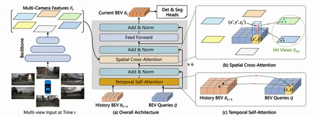
The first example is based on BEVformer, one of the more advanced BEV algorithms (Figure 4). The BEVformer algorithm reads inputs from multiple cameras (six in this example) and fuses and converts the 2D data to create a 3D BEV view. To perform the task, BEVformer relies on a mix of AI and DSP functionality. A straightforward implementation of BEVformer on the commercial solution provided measured latency of approximately 15 ms. Even lower latencies could be reached by spending some time to optimize the implementation.
Two additional implementations help put the complexity in perspective.
Example #2
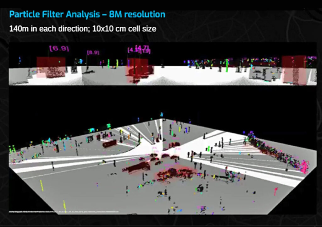
As mentioned above, a particle filter is a pure DSP implementation with no AI processing involved. As implemented on the example commercial solution, an 8 million–cell particle filter, with 16 million particles and 1.5 million new particles every cycle, provides a latency of ~6 ms. With a cell size of 10 × 10 cm, this translates to a grid map of 140 meters in all directions around the vehicle (Figure 5).
As a comparison, an implementation for a particle filter with 4 million cells and 8 million particles resulted in a latency of 100 ms when implemented on one current market leader’s hardware.
Example #3
Mask R-CNN builds on the Faster R-CNN algorithm, and the implementation requires a mix of AI and DSP. This example uses camera data provided in scene 018 of the KITTI benchmark suite. The algorithm is used to detect objects (object classes) and finds their position using bounding boxes. It also performs a pixel-oriented semantic segmentation task, placing the pixels into predefined categories. The idea is that the driver should be able to detect the position of objects even if the view is partially occluded; in Figure 6, for example, the traffic poles partially obscure the car. The algorithm is notoriously difficult to implement when the aim is to reach low latency.
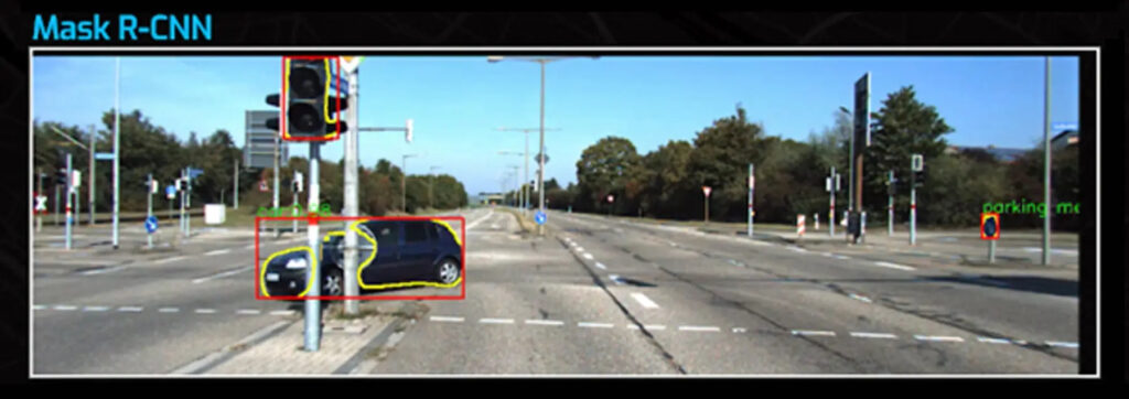
In this specific example, the implementation is running 960 × 1,280 × 3-pixel images on the commercial solution, resulting in a latency well below 10 ms. As a comparison, running Mask R-CNN on a trained Nvidia DGX A100 provides a latency of 34 ms.
If the test hardware is taken to the next step, using a chip that has a gross compute power of 512-TFLOPS AI and 8-TFLOPS DSP and combining two of the algorithms could yield a parallel implementation of an 8 million–particle filter and Mask R-CNN running with a combined latency of less than 10 ms.
The next AD evolution
The latest state-of-the-art algorithms combine AI and DSP processing. The next evolution in autonomous driving is to fuse sensor data in a 3D representation to increase the accuracy of understanding the environment and of tracking the movement of dynamic objects. The downside of these algorithms is the exceedingly high processing power requirements. The current maximum theoretical compute power reaches about 250 TOPS, inadequate for complex algorithm processing within the maximum allotted time.
One way to handle this limitation would be to increase the parallel processing of the same data in different dimensions and with different algorithms. Another way would be to reduce the amount of data to be processed without impacting the information needed for accurate perception. Tesla has tried to use cameras only, but it is now using radar as well.
An optimal solution would be to eliminate some of the higher-cost sensors. That could have a sizable impact on the total cost of ownership, as a reduced number of sensors will lower system costs and reduce the processing needs, perhaps to less than 1 POPS. On the other hand, because nature abhors a vacuum, it is a foregone conclusion that if there will be available compute power, the engineers will use it creatively.