
The automotive industry is delivering the first implementations of advanced driver-assistance systems (ADAS) for Level 2 (foot off the gas or break) and Level 3 (hands off the wheel) vehicles. Though it’s struggling to develop an autonomous driving (AD) system from L4 (eyes off the road) to L5 (completely self-driving and autonomous) vehicles. The challenge is turning out to be more difficult than anticipated a few years ago.
Implementing an AD system comes down to safely moving a vehicle from point A to point B without human assistance. This can be accomplished by a three-stage state machine called driving control loop that includes perception, motion planning, and motion execution. Perception learns and understands the driving environment, as well as the vehicle position or its localization on a map. The perception stage feeds environment and localization data to the motion or path planning that calculates the trajectory of the vehicle, in turn performed by the motion execution. If perception generates inaccurate data, the trajectory is going to be flawed. In the worst-case, it leads to catastrophic results.
A successful AD system implementation rests on a state-machine architecture that can formulate a truthful understanding of the environment, produce an efficient motion plan, and flawlessly perform its execution.
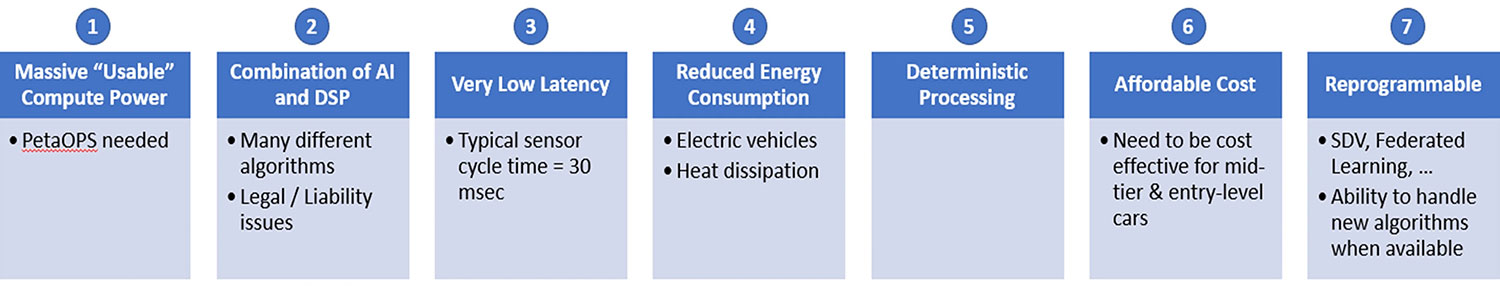
AD system’s seven essential requirements
The ideal architecture to make a viable and flawless L4 AD control loop must meet at least seven essential requirements.
First is the ability to deliver massive usable compute power in the range of PetaOps. What’s critical here is the word “usable.” What an engineer needs to know is how much of the theoretical Ops can be used at any given instance.
Second is being able to support a combination of artificial intelligence (AI) and digital signal processing (DSP). In an L4-capable vehicle, there are typically between 40 and 70 sensors for the AD functionality, including a combination of radars, LIDARs, cameras and ultrasonic sensors, in addition to the navigation data.
All these sensors generate a massive amount of data delivered in real-time. Depending on the data type, algorithmic processing may require pure AI for segmentation and object detection, for example, or pure signal processing for clustering and transforms, pre-processing of signals, fusion of signals or a combination of AI and signal processing for things like occupancy grid mapping or perception fusion.
The legal and liability aspects must be taken into consideration. Up to L3, there is always a human in charge of the vehicle. At L4, the vehicle is supposed to be in control and capable of handling the vehicle the same way a human driver would under the same circumstances.
If an L4 vehicle is involved in an accident, responsibility and liability become an issue as they move from the driver to the OEM, since there is no driver. Having the ability to prove the reliability and functionality of the AD system becomes critical. AI processing alone is not enough. The answer is to tackle the problem with a comprehensive solution.
The third requirement is to minimize latency. A typical sensor cycle time is 30 milliseconds. That means that the control loop needs to accomplish its task in 20 to 25 milliseconds to allow for a margin to handle exceptions.
Fourth is reduced energy consumption. The switch from the internal combustion engine to the electrical engine is in progress at all major car manufacturers. In a not-too-distant future, all vehicles on the road will be electrical and the focus will be to try to minimize the taxing of the battery due to massive loads.
A viable L4 AD architecture is currently expected to consume about 0.1 W per usable TeraOps, and longer term, this is expected to be further reduced. There’s also a question of heat dissipation. Automotive companies don’t want to be in a position where they need to design specific, exotic heat dissipation solutions.
Fifth is ensuring deterministic processing. For example, in a particle filter, engineers may want to do sorting. They’re not interested in what the average sort time would be, but need to know the minimum and the maximum sort times to ensure that they handle the entire loop in the allowed timing.
The sixth requirement is the need for a commercially viable cost structure to migrate from high-end vehicles to mid- and low-end classes. Today, no commercially viable L4/L5 solutions are available.
Seventh is support re-programmability. Today, the software-defined vehicle (SDV) is part of the new generation of vehicle architectures. However, re-programmability is also necessary to accommodate newer machine learning algorithms such as federated learning and others not yet on the horizon. Whatever algorithms are used today will not be the same two or three years down the road. A viable solution must be able to handle that.
Source: VSORA
Environment perception
As the vehicle is moving, objects around the vehicle move as well, forcing the driving control loop to dynamically re-calculate the motion plan. This dynamic replanning is typically handled by a local motion planner that generates an optimal trajectory using both the global planner and the surrounding environment information. That’s because there is a need to do short-term environment prediction to assess the validity of the planned trajectory.
This can be done in different ways. Namely, either via object-based representation, grid-based representation or a combination of both. The grid-based representation allows for handling complex scenarios with a large number of objects and, importantly, is less sensitive to imperfections when doing object extraction, like false or missed targets.
The dynamic occupancy grid map (DOGMa) is a grid-based representation of the local environment. It estimates the occupancy probability of an individual cell in the grid. It also takes into consideration the kinetic attributes of each cell: velocity, acceleration and turn ratio. By doing this, it allows near-future predictions of occupancy.
The DOGMa is a powerful method for performing short-term environmental prediction.
To achieve precise and stable vehicle localization in the perception stage, the vehicle’s sensors and the road infrastructure must be processed together. Given a map of the environment, a particle filter algorithm can estimate the position and orientation of an AD vehicle as it moves and senses the environment. A particle filter uses multiple samples referred to as particles to understand the object or objects that occupy a cell in the grid. Particle filters are a way to efficiently represent an arbitrary non-Gaussian distribution. Because the particles are generated randomly, they can represent the properties of non-Gaussian noise accurately if there are enough of them.
To populate the occupancy grid map, the collected sensor data for each type of sensor goes through a number of pre-processing steps such as ground identification and ray tracing. The pre-processed data is then used to create a measurement grid for each sensor type. At the end, all the measurement grids for all sensor types and the navigation data are combined into a full measurement grid that the particle filter can act on.
The particle filter captures a number of different parameters for each of the particles in an individual cell. By clustering the data, it tracks bigger objects that simplifies further processing stages and allows for handling situations where, for example, the object is partially or fully hidden.
A system based on a publicly available doctoral thesis “A Random Finite Set Approach for Dynamic Occupancy Grid Maps with Real-Time Application” is a good model. In one example, a DSP implementation uses 8 million cells, 16 million particles and one and a half-million new particles every cycle. To process this, one single-chip DSP configuration uses 1,024 ALUs running at 2 GHz.
Particle filter implementation
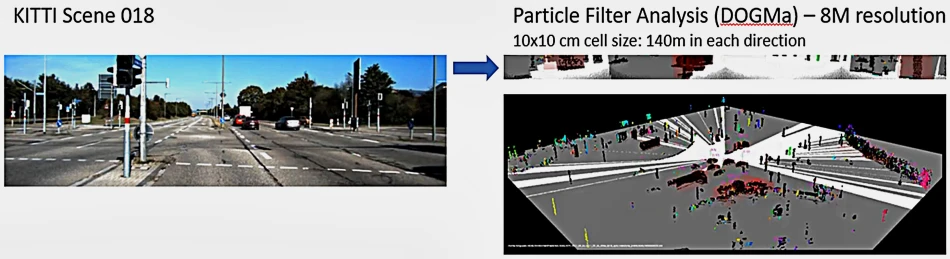
A typical commercial implementation of a particle filter would most likely use a combination of LIDAR, radar, and cameras. In this example, the chip only processes LIDAR data captured via LIDAR point clouds taken from various scenes in the KITTI database, a widely used open database originating out of the Karlsruhe Institute of Technology in Germany. Using the point cloud, the chip performs ground identification, ray tracing using Bresenham’s line algorithm, and then creates the measurement grid. Fusing additional sensors with the LIDAR data would be a straightforward task following a similar set of steps.
A grid with a 10×10 centimeter cell size was set up. For 8 million cells, the grid is 280×280 meters. The processed data, where for each cell the particles were identified and their respective velocities, shows the information in different ways. One way is show and compare the processed data video stream to the reference video. More important is the ability to create a 360-degree view, where the vehicle (the ego vehicle) sits in the center of the grid for a view of 140 meter in each direction (Figure 2).
Source: VSORA
It’s known as dynamic occupancy grid mapping. To follow the movements of vehicles and objects, the various elements of the grid have been artificially colored. Specifically, white means no obstacles on the ground. Gray means unidentified area. Black means a static object. Anything in color means dynamic object where specific colors show the direction of the movement of that object, such as yellow moving back, red turning right and blue moving forward, for example.
The top area shows the same driver’s view as the video, but the output is based on the data generated after processing through the particle filter implementation. Here the speed in meters per second of each dynamic object can also be seen.
As vehicles move, information is provided on the surrounding areas as well. More and more of the grey is changing to white, showing that this has been identified as free space. It’s not fully shaded because the particle filter performs some elements of prediction for the future or track hidden particles. If a vehicle blocks the view of another vehicle or another object, it doesn’t necessarily mean that that object is gone. It just means that it is out of view and decisions are being made on how long that object would be tracked.
Processing a particle filter is extremely computing intensive. Traditional processing engines such CPUs, GPUs and FPGAs usually don’t deliver the “useable” performance necessary for the task, and their latency exceeds the maximum allocated time for AD applications. Here, special-purpose ASICs can accomplish the demanding job.
In this case, the processing of the particle filter utilized 87% of the 1,024 ALUs, also facilitated by the high efficiency of the core native instructions of the ALUs. The overall latency is 6 milliseconds, an efficient approach to implementing an autonomous driving vehicle.
Jan Pantzar is VP of sales and marketing at VSORA, a France-based supplier of IP and chip solutions for AI and ADAS applications.
Dr. Lauro Rizzatti is a verification consultant and industry expert on hardware emulation.